When working with data we often find a need to transform it in various ways. This might be for reasons of presentation, to make data compatible with a function that requires the input to be in a specific format, or to make it easier to work with. R provides plenty of options for data transformation and the rich package system means that there is typically a ready made solution for most of the problems that you might encounter.
Wide and long format transformations
Consider the following dataset;
dat <- data.frame(
    first_name = c("Olivia", "Amelia", "George"),
    post_code = c("AB12CD", "EF34GH", "IJ56KL"),
    hair_colour = c("brown", "brown", "blond"),
    eye_colour = c("green", "blue", "blue")
)

print(dat)
#'   first_name post_code hair_colour eye_colour
#' 1     Olivia    AB12CD       brown      green
#' 2     Amelia    EF34GH       brown       blue
#' 3     George    IJ56KL       blond       blue
The data has one row per individual and records their name, post code, hair colour, and eye colour. Each observation is held in a column and the layout could be described as being a wide format.
The same data could also be stored in a long format where the post code, hair colour, and eye colour are all stored in a single column of values, with another column used to identify what the value signifies.
Wide format
| first_name | post_code | hair_colour | eye_colour |
|---|---|---|---|
| Olivia | AB12CD | brown | green |
| Amelia | EF34GH | brown | blue |
| George | IJ56KL | blond | blue |
Long format
| first_name | measure | value |
|---|---|---|
| Olivia | post_code | AB12CD |
| Amelia | post_code | EF34GH |
| George | post_code | IJ56KL |
| Olivia | hair_colour | brown |
| Amelia | hair_colour | brown |
| George | hair_colour | blond |
| Olivia | eye_colour | green |
| Amelia | eye_colour | blue |
| George | eye_colour | blue |
Wide to Long transformation
Whilst there are a number of functions available to assist in the wide to long transformation, pivot_longer from the tidyr package offers one of the simpler API’s. tidyr is a widely used package and the pivot_longer function is performant with small to mid sized data.
You can install tidyr from CRAN if you don’t already have it installed.
install.packages("tidyr")To use pivot_longer to transform our data we need to specify at least the data and cols arguments. data allows us to specify the object that we want to transform, and cols specifies the columns to pivot into the longer format.
tidyr::pivot_longer(data = dat, cols = c(post_code, hair_colour, eye_colour))
#' # A tibble: 9 × 3
#'   first_name name        value
#'   <chr>      <chr>       <chr>
#' 1 Olivia     post_code   AB12CD
#' 2 Olivia     hair_colour brown
#' 3 Olivia     eye_colour  green
#' 4 Amelia     post_code   EF34GH
#' 5 Amelia     hair_colour brown
#' 6 Amelia     eye_colour  blue
#' 7 George     post_code   IJ56KL
#' 8 George     hair_colour blond
#' 9 George     eye_colour  blue
We can also use negation in the cols argument; in our example we actually want to pivot all columns except first_name, so we can also write the function like this;
tidyr::pivot_longer(data = dat, cols = !first_name)
#' # A tibble: 9 × 3
#'   first_name name        value
#'   <chr>      <chr>       <chr>
#' 1 Olivia     post_code   AB12CD
#' 2 Olivia     hair_colour brown
#' 3 Olivia     eye_colour  green
#' 4 Amelia     post_code   EF34GH
#' 5 Amelia     hair_colour brown
#' 6 Amelia     eye_colour  blue
#' 7 George     post_code   IJ56KL
#' 8 George     hair_colour blond
#' 9 George     eye_colour  blue
You will have noticed that the return of pivot_longer is a tibble. This generally won’t be a problem, but we can keep our data in a data.frame by using as.data.frame() to wrap our call to pivot_longer(), for example as.data.frame(tidyr::pivot_longer(data, cols)).
Typically, we might want to specify the names of the new name and value columns rather than using the default values. This can be achieved with the names_to and values_to arguments.
as.data.frame(
    tidyr::pivot_longer(
        data = dat,
        cols = !first_name,
        names_to = "measure", values_to = "value"
        )
    )
#'   first_name     measure  value
#' 1     Olivia   post_code AB12CD
#' 2     Olivia hair_colour  brown
#' 3     Olivia  eye_colour  green
#' 4     Amelia   post_code EF34GH
#' 5     Amelia hair_colour  brown
#' 6     Amelia  eye_colour   blue
#' 7     George   post_code IJ56KL
#' 8     George hair_colour  blond
#' 9     George  eye_colour   blue
The function has worked well so far, but what if we had another column containing numeric values that we also wanted to include in the transformation?
dat$age <- c(64, 25, 56)

as.data.frame(
    tidyr::pivot_longer(
        data = dat,
        cols = !first_name,
        names_to = "measure", values_to = "value"
        )
    )
#' Error in `pivot_longer_spec()`:
#' ! Can't combine `post_code` <character> and `age` <double>.
#' Run `rlang::last_error()` to see where the error occurred.
Our post_code, hair_colour, and eye_colour columns were all character vectors, whereas our newly added age column is numeric. tidyverse functions usually try to avoid implicit type coercions, so whilst you might have expected age to be coerced into a character, we have instead received an error.
We can use the values_transform argument to specify the as.character function, which will then be applied to all columns in the transformation.
dat$age <- c(64, 25, 56)

dat <- as.data.frame(
    tidyr::pivot_longer(
        data = dat,
        cols = !first_name,
        names_to = "measure", values_to = "value",
        values_transform = as.character
        )
    )

print(dat)
#'    first_name     measure  value
#' 1      Olivia   post_code AB12CD
#' 2      Olivia hair_colour  brown
#' 3      Olivia  eye_colour  green
#' 4      Olivia         age     64
#' 5      Amelia   post_code EF34GH
#' 6      Amelia hair_colour  brown
#' 7      Amelia  eye_colour   blue
#' 8      Amelia         age     25
#' 9      George   post_code IJ56KL
#' 10     George hair_colour  blond
#' 11     George  eye_colour   blue
#' 12     George         age     56
Note that we wrote values_transform = as.character and not values_transform = as.character(). The reasons for this are to do with how the pivot_longer function is written internally, but for now it is sufficient to have this pointed out.
pivot_longer offers a range of arguments allowing the user to exert varying levels of control over the transformation that takes place. You can view the documentation by running ?pivot_longer.
Long to Wide transformation
pivot_wider from the tidyr package is used for transforming data from a long to wide format. Having used pivot_longer, it should feel somewhat familiar.
We can use pivot_wider to return our data.frame, dat back to a wide format. dat currently looks like this;
| first_name | measure | value |
|---|---|---|
| Olivia | post_code | AB12CD |
| Olivia | hair_colour | brown |
| Olivia | eye_colour | green |
| Olivia | age | 64 |
| Amelia | post_code | EF34GH |
| Amelia | hair_colour | brown |
| Amelia | eye_colour | blue |
| Amelia | age | 25 |
| George | post_code | IJ56KL |
| George | hair_colour | blond |
| George | eye_colour | blue |
| George | age | 56 |
The minimum arguments that we need to provide to transform our data with pivot_wider are names_from (the column values will be converted to the column names) and values_from (the values that will populate the new columns). We also need to pass our data.frame as the data argument.
as.data.frame(
    tidyr::pivot_wider(
        data = dat,
        names_from = measure,
        values_from = value
        )
)
#'   first_name post_code hair_colour eye_colour age
#' 1     Olivia    AB12CD       brown      green  64
#' 2     Amelia    EF34GH       brown       blue  25
#' 3     George    IJ56KL       blond       blue  56
pivot_wider also offers a range of additional arguments allowing the user to exert control over the transformation that takes place. You can view the documentation by running ?pivot_wider.
Joins
Joining two datasets together is a powerful technique, typically used to combine rows from two or more tables, based on a related column between them.
Let’s use an example of 2 tables; employees and skills. Both tables contain details of a unique identifier (uid), which is used to identify individual employees.
employees also contains details of an employees job role (role) and length of service in years (service).
skills contains 2 columns, python and r, used to record whether an employee knows those languages. Managers don’t do anything practical (obviously) so nobody bothered to record their programming skills, hence they don’t appear in the skills data.
employees <- data.frame(
    uid = c("001", "002", "003", "004", "005"),
    role = c("data scientist", "data scientist", "data engineer", "data scientist", "manager"),
    service = c(1,3,4,5,3)
)

skills <- data.frame(
    uid = c("001", "002", "003", "004"),
    python = c(TRUE, TRUE, FALSE, TRUE),
    r = c(TRUE, FALSE, TRUE, TRUE)
)
We can use the merge function to perform a wide range of different joins. Whatever the type of join required, much of the syntax remains the same. The x and y arguments are used to specify the two data.frame’s to be joined and by is used to specify the columns which the merge will be performed on.
Inner join
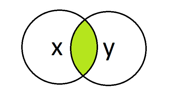
Inner joins are used to join data but keep only the rows where the merge column value exists in both x and y.
merge(x = employees, y = skills, by = c("uid"))
#'   uid           role service python     r
#' 1 001 data scientist       1   TRUE  TRUE
#' 2 002 data scientist       3   TRUE FALSE
#' 3 003  data engineer       4  FALSE  TRUE
#' 4 004 data scientist       5   TRUE  TRUE
Employee ‘005’ doesn’t appear in the returned data.frame as “005” only existed in x.
Outer join
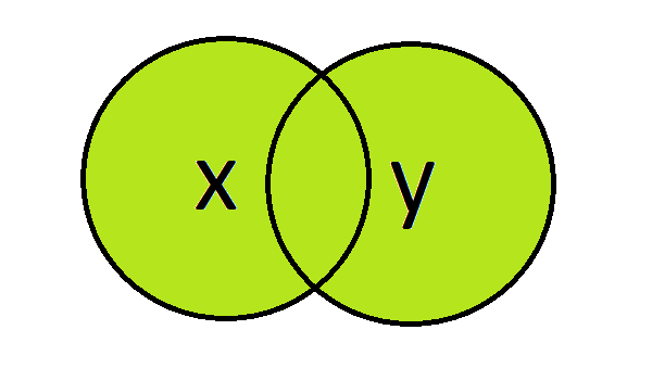
The outer join is used to join the datasets whilst keeping all records from x and y. We set the all argument to TRUE to perform this join.
merge(x = employees, y = skills, by = c("uid"), all = TRUE)
#'   uid           role service python     r
#' 1 001 data scientist       1   TRUE  TRUE
#' 2 002 data scientist       3   TRUE FALSE
#' 3 003  data engineer       4  FALSE  TRUE
#' 4 004 data scientist       5   TRUE  TRUE
#' 5 005        manager       3     NA    NA
All records from x and y are included in the return, however, as employee ‘005’ did not exist in y the values for that employee in the python and r column have been set to NA.
Left join
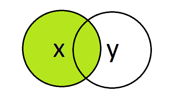
A left join returns all rows from the left table (x) and matched rows from the right table (y).
merge(x = employees, y = skills, by = c("uid"), all.x = TRUE)
#'   uid           role service python     r
#' 1 001 data scientist       1   TRUE  TRUE
#' 2 002 data scientist       3   TRUE FALSE
#' 3 003  data engineer       4  FALSE  TRUE
#' 4 004 data scientist       5   TRUE  TRUE
#' 5 005        manager       3     NA    NA
This time the return includes employee ‘005’ as the row existed in the left table (x) and again the values in the python and r columns have been set to NA as there was no row for the employee in the right table (y).
Right join
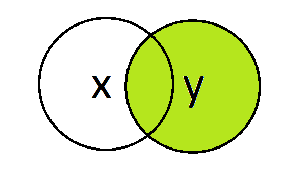
A right join returns matched rows from the left table (x) and all rows from the right table (y).
merge(x = employees, y = skills, by = c("uid"), all.y = TRUE)
#'   uid           role service python     r
#' 1 001 data scientist       1   TRUE  TRUE
#' 2 002 data scientist       3   TRUE FALSE
#' 3 003  data engineer       4  FALSE  TRUE
#' 4 004 data scientist       5   TRUE  TRUE
This time the return does not include employee ‘005’ as the row existed only in the left table (x).
Summary
The merge() function provides a simple and intuitive API. In the examples above the x, y, and by arguments remain the same across the different types of join. The table below demonstrates the additional arguments required to achieve each type of join.
| inner join | outer join | left join | right join |
|---|---|---|---|
|
|
|
|
| all = FALSE | all = TRUE | all.x = TRUE | all.y = TRUE |
A tidy approach
The tidyverse package dplyr provides functions for performing joins on a pair of data.frames.
Inner join
dplyr::inner_join(x = employees, y = skills, by = c("uid"))
#'   uid           role service python     r
#' 1 001 data scientist       1   TRUE  TRUE
#' 2 002 data scientist       3   TRUE FALSE
#' 3 003  data engineer       4  FALSE  TRUE
#' 4 004 data scientist       5   TRUE  TRUE
Outer join
dplyr::full_join(x = employees, y = skills, by = c("uid"))
#'   uid           role service python     r
#' 1 001 data scientist       1   TRUE  TRUE
#' 2 002 data scientist       3   TRUE FALSE
#' 3 003  data engineer       4  FALSE  TRUE
#' 4 004 data scientist       5   TRUE  TRUE
#' 5 005        manager       3     NA    NA
Left join
dplyr::left_join(x = employees, y = skills, by = c("uid"))
#'   uid           role service python     r
#' 1 001 data scientist       1   TRUE  TRUE
#' 2 002 data scientist       3   TRUE FALSE
#' 3 003  data engineer       4  FALSE  TRUE
#' 4 004 data scientist       5   TRUE  TRUE
#' 5 005        manager       3     NA    NA
Right join
dplyr::right_join(x = employees, y = skills, by = c("uid"))
#'   uid           role service python     r
#' 1 001 data scientist       1   TRUE  TRUE
#' 2 002 data scientist       3   TRUE FALSE
#' 3 003  data engineer       4  FALSE  TRUE
#' 4 004 data scientist       5   TRUE  TRUE
Next steps
The data transformation techniques discussed here are powerful and effective techniques, whilst being simple to use. They are particularly useful in analytical based projects.
Try out some of the tasks below to put the theory into practice.
The below code can be used to generate 2 data.frame’s, transfers and cl_goals. transfers contains data pertaining to the most expensive association football transfers (as of Summer 2021). cl_goals contains data of the 50 all time champions league top scorers (as of 2nd November 2022).
transfers <- structure(list(player_uid = c(1L, 1L, 1L, 1L, 1L, 1L, 2L, 2L,
2L, 2L, 2L, 2L, 3L, 3L, 3L, 3L, 3L, 3L, 4L, 4L, 4L, 4L, 4L, 4L,
5L, 5L, 5L, 5L, 5L, 5L, 6L, 6L, 6L, 6L, 6L, 6L, 7L, 7L, 7L, 7L,
7L, 7L, 8L, 8L, 8L, 8L, 8L, 8L, 9L, 9L, 9L, 9L, 9L, 9L, 10L,
10L, 10L, 10L, 10L, 10L), measure = c("Player", "FromClub",
"ToClub", "Position", "FeeEuro", "FeePound", "Player",
"FromClub", "ToClub", "Position", "FeeEuro", "FeePound",
"Player", "FromClub", "ToClub", "Position", "FeeEuro",
"FeePound", "Player", "FromClub", "ToClub", "Position",
"FeeEuro", "FeePound", "Player", "FromClub", "ToClub",
"Position", "FeeEuro", "FeePound", "Player", "FromClub",
"ToClub", "Position", "FeeEuro", "FeePound", "Player",
"FromClub", "ToClub", "Position", "FeeEuro", "FeePound",
"Player", "FromClub", "ToClub", "Position", "FeeEuro",
"FeePound", "Player", "FromClub", "ToClub", "Position",
"FeeEuro", "FeePound", "Player", "FromClub", "ToClub",
"Position", "FeeEuro", "FeePound"), value = c("Neymar",
"Barcelona", "Paris Saint-Germain", "Forward", "222", "£198",
"Kylian Mbappé", "Monaco", "Paris Saint-Germain", "Forward",
"180", "£163", "Philippe Coutinho", "Liverpool", "Barcelona",
"Midfielder", "145", "£105", "João Félix", "Benfica", "Atlético Madrid",
"Forward", "126", "£104.10", "Antoine Griezmann", "Atlético Madrid",
"Barcelona", "Forward", "120", "£107", "Jack Grealish", "Aston Villa",
"Manchester City", "Midfielder", "117", "£100", "Paul Pogba",
"Juventus", "Manchester United", "Midfielder", "105", "£89",
"Ousmane Dembélé", "Borussia Dortmund", "Barcelona", "Forward",
"105", "£97", "Gareth Bale", "Tottenham Hotspur", "Real Madrid",
"Forward", "100", "£86", "Cristiano Ronaldo", "Real Madrid",
"Juventus", "Forward", "100", "£88")), row.names = c(2L, 3L,
4L, 5L, 6L, 7L, 9L, 10L, 11L, 12L, 13L, 14L, 16L, 17L, 18L, 19L,
20L, 21L, 23L, 24L, 25L, 26L, 27L, 28L, 30L, 31L, 32L, 33L, 34L,
35L, 37L, 38L, 39L, 40L, 41L, 42L, 44L, 45L, 46L, 47L, 48L, 49L,
51L, 52L, 53L, 54L, 55L, 56L, 58L, 59L, 60L, 61L, 62L, 63L, 65L,
66L, 67L, 68L, 69L, 70L), class = "data.frame")

cl_goals <- structure(list(Rank = c(1L, 2L, 3L, 4L, 5L, 6L, 7L, 8L, 9L, 10L,
10L, 12L, 12L, 14L, 15L, 15L, 17L, 18L, 19L, 20L, 21L, 22L, 23L,
24L, 25L, 25L, 25L, 25L, 25L, 30L, 30L, 30L, 33L, 33L, 33L, 33L,
37L, 37L, 37L, 40L, 40L, 42L, 42L, 42L, 45L, 45L, 45L, 45L, 45L,
45L, 45L), Player = c("Cristiano Ronaldo", "Lionel Messi",
"Robert Lewandowski", "Karim Benzema", "Raúl", "Ruud van Nistelrooy",
"Thomas Müller", "Thierry Henry", "Alfredo Di Stéfano ",
"Andriy Shevchenko", "Zlatan Ibrahimović", "Eusébio ",
"Filippo Inzaghi", "Didier Drogba", "Mohamed Salah", "Neymar",
"Alessandro Del Piero", "Sergio Agüero", "Kylian Mbappé",
"Ferenc Puskás", "Edinson Cavani", "Gerd Müller",
"Fernando Morientes", "Arjen Robben", "Samuel Eto'o", "Antoine Griezmann",
"Wayne Rooney", "Kaká", "Francisco Gento", "David Trezeguet",
"Roy Makaay", "Patrick Kluivert", "Erling Haaland", "Jean-Pierre Papin",
"Edin Džeko", "Ryan Giggs", "Sadio Mané", "Luis Suárez",
"Rivaldo", "Mario Gómez", "Raheem Sterling", "Mário Jardel",
"Robin van Persie", "Hernán Crespo", "José Altafini ",
"Marco Simone ", "José Augusto ", "Giovane Élber",
"Gonzalo Higuaín", "Luís Figo", "Paul Scholes"), Goals = c(140L,
129L, 91L, 86L, 71L, 56L, 53L, 50L, 49L, 48L, 48L, 46L, 46L,
44L, 43L, 43L, 42L, 41L, 40L, 36L, 35L, 34L, 33L, 31L, 30L, 30L,
30L, 30L, 30L, 29L, 29L, 29L, 28L, 28L, 28L, 28L, 27L, 27L, 27L,
26L, 26L, 25L, 25L, 25L, 24L, 24L, 24L, 24L, 24L, 24L, 24L),
    Apps = c(183L, 161L, 111L, 146L, 142L, 73L, 138L, 112L, 58L,
    100L, 124L, 65L, 81L, 92L, 77L, 80L, 89L, 79L, 59L, 41L,
    70L, 35L, 93L, 110L, 78L, 85L, 85L, 86L, 89L, 58L, 61L, 71L,
    23L, 37L, 68L, 145L, 61L, 73L, 73L, 44L, 79L, 46L, 59L, 65L,
    28L, 46L, 56L, 69L, 83L, 103L, 124L)), class = "data.frame", row.names = c(NA,
-51L))
The transfers dataset is in a long format, consisting of 3 columns, player_uid, measure, and value. Transform the dataset into a wide format, the transformed dataset should contain the columns;
- player_uid
- Player
- FromClub
- ToClub
- Position
- FeeEuro
- FeePound
Join the transfers and cl_goals datasets using the Player column to create a new dataset named tg containing only the players that are present in both datasets.
Using the tg dataset you have created;
-
How many players are included in
tg? -
What is the combined number of Champions League appearences made by players in
tg? -
Which player scored the most goals per Champions League appearence?
-
Considering the fee paid for each player in euro’s, calculate the spend per Champions League goal and assign the result to a column named
spend_per_goal. Which player had the lowest spend per Champions League goal?
hint: some columns may not be numeric, as.numeric() can be used to change type
Answers
1. 42. 407
3. Cristiano Ronaldo
4. Cristiano Ronaldo