Before we can start working with data we need to import it into the R environment. Base R (the language as installed without any additional libraries) provides a number of functions for reading data in multiple formats, but the performance benefits and ease of use of some functions provided by external libraries makes them the go to choice for many users.
The following examples cover reading some of the most common types of data into R. Whilst by no means an exhaustive list of all the available options, the functions detailed are performant, stable, and easy to use.
CSV
One of the most common cross-platform methods for storing typically tabular data.
readr::read_csv()
The tidyverse package readr offers the read_csv() function. It’s relatively performant, it makes a good job of inferring types, and for users planning to use the tidyverse it helpfully returns a tibble.
During interactive use calling the function prints some useful information regarding the delimiter used and column types detected.
dat <- readr::read_csv("example_path/example.csv")
#' Rows: 5 Columns: 4
#' ── Column specification
#' Delimiter: ","
#' chr  (1): uid
#' dbl  (2): col_a, col_b
#' date (1): date
#'
#' ℹ Use `spec()` to retrieve the full column specification for this data.
#' ℹ Specify the column types or set `show_col_types = FALSE` to quiet this message.

print(dat)
#' # A tibble: 5 × 4
#' uid   date        col_a    col_b
#' <chr> <date>      <dbl>    <dbl>
#' 1 a     2022-08-01 -0.308 -0.943
#' 2 b     2022-08-01  0.695  0.0587
#' 3 c     2022-08-01  1.15  -0.621
#' 4 d     2022-08-01  0.245 -1.41
#' 5 e     2022-08-01  0.448  0.00618
read_csv is fast, predictable, and stable. The additional information provided can be useful during interactive analysis. The readr package is very widely used and is actively maintained and developed, providing some confidence for developers aiming for long term reproducibility.
A full list of read_csv’s arguments can be found by running ?readr::read_csv.
data.table::fread()
When performance and speed is of the utmost importance nothing really comes close to the data.table package. The fread() function is simple to use, blazingly fast, and the 10,000 row sample it takes of equally spaced data throughout the target file allows it to make very accurate guesses at column type.
dat <- data.table::fread("example_path/example.csv")

print(dat)
#'    uid       date      col_a        col_b
#' 1:   a 2022-08-01 -0.3082584 -0.942751791
#' 2:   b 2022-08-01  0.6946568  0.058719041
#' 3:   c 2022-08-01  1.1463694 -0.621216248
#' 4:   d 2022-08-01  0.2453974 -1.408545363
#' 5:   e 2022-08-01  0.4482430  0.006183595

sapply(dat, class)
#'         uid             date        col_a       col_b
#' "character"   "IDate" "Date"     "double"    "double"
fread returns a data.table class object by default, however, we can easily have the function return a data.frame by passing the argument data.table=FALSE. data.table’s can be used anywhere you would use a data.frame.
class(data.table::fread("example_path/example.csv"))
#' [1] "data.table" "data.frame"

class(data.table::fread("example_path/example.csv", data.table=FALSE))
#' [1] "data.frame"
The data.table package is widely used and is actively maintained and developed, like with readr this provides some confidence for developers aiming for long term reproducibility. Given its speed data.table is a good option for any process going into a production environment and long running work flows.
A full list of fread’s arguments can be found by running ?data.table::fread.
Which should I use?
readr::read_csv() and data.table::fread() are both solid choices for reading a CSV file. The most pressing factors may come down to speed and the packages you intend to use for the rest of your process. If relying heavily upon the tidyverse it makes sense to lean toward readr, whereas when working with large datasets data.table will likely make more sense.
XLSX
The ubiquitous format for excel spreadsheets since 2007. Still pervasively popular and sometimes misused despite a wide array of alternatives. Being able to confidently read .xlsx files will definitely be come in handy.
openxlsx::read.xlsx()
openxlsx is a well established package, with fewer dependencies than some of the alternatives (no Java dependency). The read.xlsx() function is straightforward to use.
dat <- openxlsx::read.xlsx("example_path/example.xlsx")

print(dat)
#'   uid  date      col_a        col_b
#' 1   a 44774 -0.3082584 -0.942751791
#' 2   b 44774  0.6946568  0.058719041
#' 3   c 44774  1.1463694 -0.621216248
#' 4   d 44774  0.2453974 -1.408545363
#' 5   e 44774  0.4482430  0.006183595
Dates can sometimes be read as integers when reading .xlsx files, but this is easily overcome by supplying the argument detectDates=TRUE. Generally, the column type detection is adequate.
dat <- openxlsx::read.xlsx("example_path/example.xlsx", detectDates=TRUE)

print(dat)
#'   uid       date      col_a        col_b
#' 1   a 2022-08-01 -0.3082584 -0.942751791
#' 2   b 2022-08-01  0.6946568  0.058719041
#' 3   c 2022-08-01  1.1463694 -0.621216248
#' 4   d 2022-08-01  0.2453974 -1.408545363
#' 5   e 2022-08-01  0.4482430  0.006183595

sapply(dat, class)
#'         uid        date       col_a       col_b
#' "character"      "Date"   "numeric"   "numeric"
When working with excel workbooks we often find notes or titles contained in the first few lines of a worksheet, followed by the tabular data we want to import. We may also have workbooks containing multiple worksheets, where only specific worksheets are of interest.
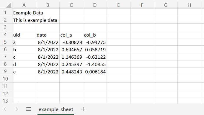
openxlsx::read.xlsx() makes it easy for us to specify and read data from specific worksheets and cell ranges.
openxlsx::read.xlsx("example_path/example.xlsx", sheet="example_sheet", cols=c(1:4), rows(4:9))A full list of read.xlsx’s arguments can be found by running ?openxlsx::read.xlsx.
RDS
readRDS()
One of R’s own formats for storing data, RDS files store a single R object. Reading them is achieved with the base function readRDS.
dat <- readRDS("example_path/example.RDS")

print(dat)
#'   uid       date      col_a        col_b
#' 1   a 2022-08-01 -0.3082584 -0.942751791
#' 2   b 2022-08-01  0.6946568  0.058719041
#' 3   c 2022-08-01  1.1463694 -0.621216248
#' 4   d 2022-08-01  0.2453974 -1.408545363
#' 5   e 2022-08-01  0.4482430  0.006183595
An RDS file captures the state of an object and as such each column of our data reads in with the same type and class attributes as when it was created.
A full list of readRDS’s arguments can be found by running ?readRDS.
ZIP
ZIP is an archive format used for data compression. A ZIP file can contain multiple files and even directories that have been compressed, however, we may often encounter a ZIP file containing a single CSV file.
We have a couple of options for unzipping and reading the CSV for which we welcome back the readr and data.table packages.
readr::read_csv()
readr offers the simplest option with the read_csv function, it detects that the target is compressed and using its internal method dispatch handles the unzip and import.
readr::read_csv("example_path/example.zip")
#' Rows: 5 Columns: 4
#' ── Column specification
#' Delimiter: ","
#' chr  (1): uid
#' dbl  (2): col_a, col_b
#' date (1): date
#'
#' ℹ Use `spec()` to retrieve the full column specification for this data.
#' ℹ Specify the column types or set `show_col_types = FALSE` to quiet this message.

print(dat)
#' # A tibble: 5 × 4
#' uid   date        col_a    col_b
#' <chr> <date>      <dbl>    <dbl>
#' 1 a     2022-08-01 -0.308 -0.943
#' 2 b     2022-08-01  0.695  0.0587
#' 3 c     2022-08-01  1.15  -0.621
#' 4 d     2022-08-01  0.245 -1.41
#' 5 e     2022-08-01  0.448  0.00618
data.table::fread()
The data.table option once again uses fread. The usage is a little more complex but is also highly customizable. We can use the cmd argument to pass a shell command to handle the preprocessing of the target file.
Our shell command will contain;
unzipto extract the file-pan option to extract files to stdoutexample.zipthe path to the target file
dat <- data.table::fread(cmd = "unzip -p example_path/example.zip")

print(dat)
#'  uid       date      col_a        col_b
#' 1   a 2022-08-01 -0.3082584 -0.942751791
#' 2   b 2022-08-01  0.6946568  0.058719041
#' 3   c 2022-08-01  1.1463694 -0.621216248
#' 4   d 2022-08-01  0.2453974 -1.408545363
#' 5   e 2022-08-01  0.4482430  0.006183595
JSON
jsonlite::fromJSON()
JSON (JavaScript Object Notation) is a standardized file format used to store key value attributes in a format specifically designed to be human readable. It is commonly used for configuration files and transmitting data over the internet.
We can read JSON files using fromJSON from the jsonlite package.
jsonlite::fromJSON("example_path/example.json")
#' $value_a
#' [1] 123
#'
#' $value_b
#' [1] 123
#'
#' $value_c
#' [1] "abc"
A full list of fromJSON’s arguments can be found by running ?jsonlite::fromJSON.
YAML
yaml::yaml.load_file()
YAML (Yet Another Markup Language YAML Ain’t Markup Language) is another format commonly used for configuration files.
We can read YAML using the yaml.load_file function from the yaml package.
yaml::yaml.load_file("example_path/example.yaml")
#' $value_a
#' [1] 123
#'
#' $value_b
#' [1] 123
#'
#' $value_c
#' [1] "abc"
A full list of yaml.load_file’s arguments can be found by running ?yaml::yaml.load_file.
RData
load()
Another format specific to R, RData can be used to store a complete workspace or selected objects. Its a less widely used format, but simple enough to read using the base function load. The load function is a little different to the other examples given as we don’t assign its output, rather the function loads the objects contained within the RData file straight into out environment.
exists("example")
#' [1] FALSE

load("example_path/example.RData") # example.RData contains an object named example

exists("example")
#' [1] TRUE
A full list of load’s arguments can be found by running ?load.
Proprietary formats
The haven package provides functionality for reading a number of proprietary file formats, including those used by SPSS, SAS, and Stata. The full package documentation provides further details.
To read a SPSS SAV file we can use the package’s read_sav function. Being a part of the tidyverse family, haven functions return a tibble.
dat <- haven::read_sav('example_path/example.sav')

print(dat)
#' # A tibble: 5 × 4
#' uid   date        col_a    col_b
#' <chr> <date>      <dbl>    <dbl>
#' 1 a     2022-08-01 -0.308 -0.943
#' 2 b     2022-08-01  0.695  0.0587
#' 3 c     2022-08-01  1.15  -0.621
#' 4 d     2022-08-01  0.245 -1.41
#' 5 e     2022-08-01  0.448  0.00618#
Next Steps
The above functions will allow us to read many of the most commonly encountered file types used for storing data. The R community is very active in developing solutions to common challenges and packages exist for reading data from many more sources than those covered here. Stack Overflow and the rstats subreddit are often useful resources for browsing solutions and asking questions.