Introduction to RStudio

In terms of famous duos, neither Tom and Jerry, nor Mario and Luigi, have anything on R and RStudio. The two are so commonly used together that many beginners may initially struggle to understand where one starts and the other ends.

Despite the association though, RStudio is definitely not R, in fact R doesn’t even come bundled with RStudio. Rather RStudio is an Integrated Development Environment (IDE) which aims to make working with R easier.

RStudio is available in both open source and commercial flavours, though much of the functionality is the same for end users, with the paid versions tending to offer more configuration options behind the scenes.

Getting Started

This guide assumes that you have access to RStudio, either installed locally, or in the cloud, and that this is your first time using it. If you have already used RStudio, however, you should still find some useful hints and tips.

Default settings

The default settings for RStudio are sufficient in most cases, however, there are a few settings that I recommend nearly all users change.

Click Tools > Global Options
Navigate to the General heading from the sidebar, and the Basic tab.
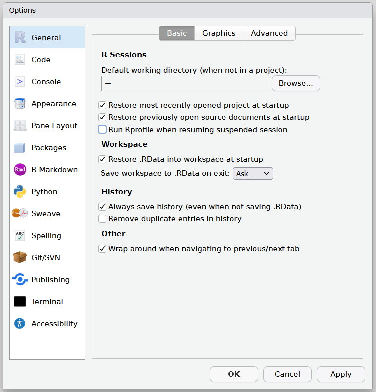
Untick;

3.1 Restore most recently opened project at startup

3.2 Restore previously open source documents at startup

3.3 Restore .RData into workspace at startup

3.4 Always save history (even when not saving .RData)
Change the dropdown for Save workspace to .RData on exit: from Ask to Never

Default settings	Recommended settings

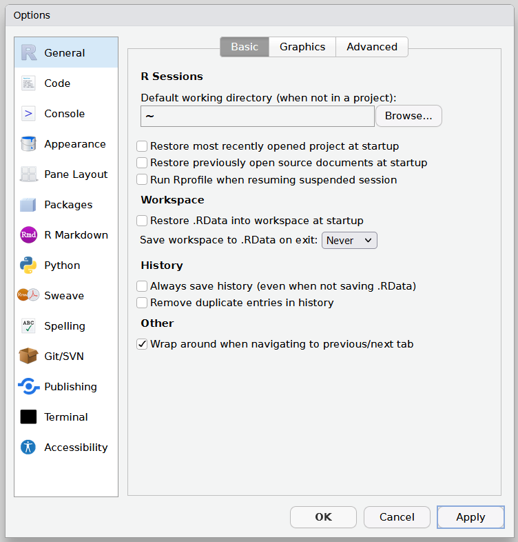These options all relate to whether RStudio will attempt to save and reload your working environment when you close and reopen it. Whilst this would be welcome if it related to scripts alone, it also attempts to save any objects you have created which can sometimes mean multiple gigabytes worth of data. It is nearly always preferable, therefore, to turn this functionality off except for a few edge cases.

Another couple of options worth changing can be found under Code > Editing, and Code > Display, where we can enable Use native pipe operator and Use rainbow parentheses.

The native pipe operator |> is the native R replacement for %>% from the magrittr package. However, it does require R version 4.1+ and a newer version of RStudio.

Rainbow parentheses are also only available in newer versions of RStudio and colour match opening and closing parentheses in an attempt to make it easier to identify pairs.

Appearance

The default appearance of RStudio is a little dated, and its certainly not one of the prettiest applications out there. Thankfully, that has little impact on its functionality, however, making a few adjustments can drastically improve the look and feel of RStudio and the dark themes certainly help ease long days staring at a screen.

To select a font and theme you can click Tools > Global Options > Appearance and browse through the available options.

Pane layout

Panes refer to the layout of the RStudio application, which typically divides the screen into four sections, each one being a pane. The layout of the panes can be configured to match your personal preferences.

Like the appearance settings, each person will have their own preference, but experimenting and finding a set-up that feels right for you can make a huge difference to how intuitive your overall experience of using RStudio becomes.

You can change the layout by clicking on the square that looks a little like a waffle and selecting Pane Layout… from the context menu. Alternatively, you can access the same options through Tools > Global Options > Pane Layout.

The settings Pane Layout section is handily divided up into four squares, the drop down menu in each can be used to specify what is displayed there, and the tick boxes beneath allow you to further shuffle around some of the sub options.

Additional columns

Adding an additional column allows us to have two scripts open side by side. It again requires clicking on the little waffle and selecting Pane Layout… or navigating through Tools > Global Options > Pane Layout.

Then its as simple as clicking Add Column. To remove the column again you can either navigate back to the same place and click Remove Column, or close all of the tabs open in the column, in which case it will disappear on its own.

There is of course an easier way to add a column, using the keyboard shortcut CTRL + F7.

Useful tabs

Within the four pane layout there are multiple useful tabs. The exact location of these can be configured to your liking. Many of these tabs provide functionality for interacting with your R environment or operating system in a way that makes using R more interactive.

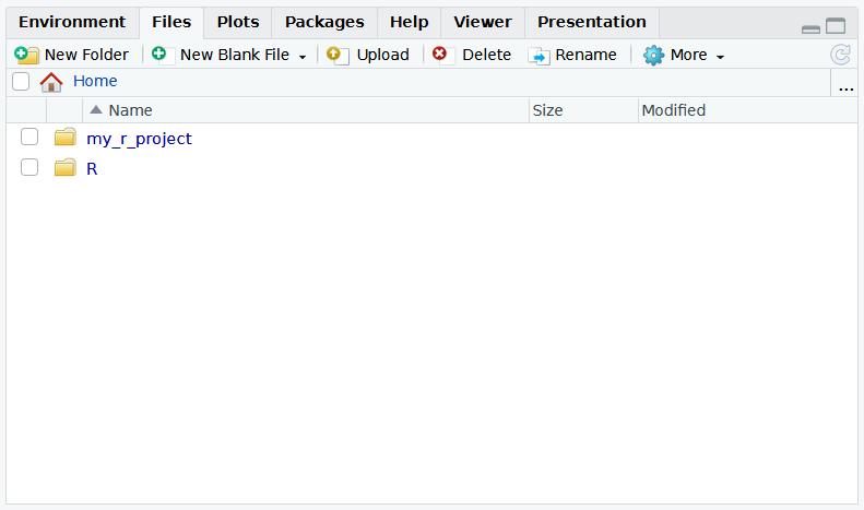
Files

The Files tab provides a minimally featured file manager and provides a handy way to perform common tasks without leaving RStudio. This can be particularly useful when working in the cloud where you may not have access to the remote machine directly.

Using the buttons in the top tool bar, you can;

Create a new folder
Create a new file
Upload a file from your local device
Delete a file
Rename a file

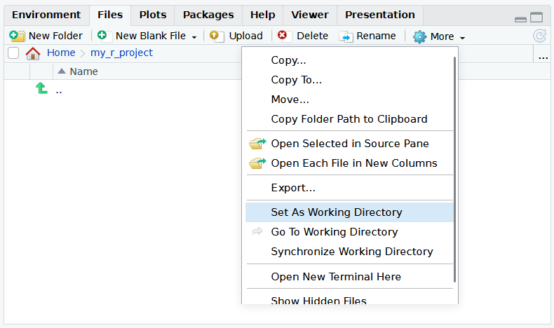
Clicking More reveals some further actions. One useful function is Set As Working Directory, which sets the working directory to the folder location currently open in Files.

Creating new files

In addition to using the New Blank File option within the Files tab, there are a few other ways to create a new files.

The quickest is the keyboard shortcut CTRL + SHIFT + N.

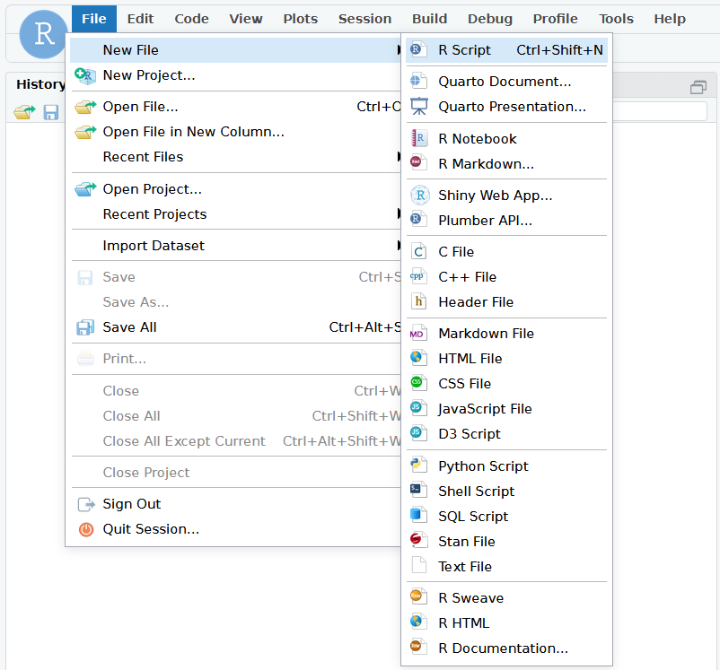
You can also use the main menu, File > New File > R Script. A number of file types can be chosen using this option. The exact file types available vary dependent upon the version of RStudio you are running.

Saving files can be done in a few ways, using the main menus File > Save, by clicking on the save icons, or with the keyboard shortcut CTRL + S. The Save All option (two disk icon) is also helpful and saves all open tabs; the keyboard shortcut is CTRL + ALT + S.

Setting the working directory

The term folder may be more familiar to Windows users, but the terms directory and folder are typically used interchangeably. The concept of setting a working directory is like saying “until I say otherwise, all the files I mention are in this particular directory”.

For example, setting the working directory to /a/very/long/path/to/my_r_project/, allows us to replace

/a/very/long/path/to/my_r_project/my_script_1.R

with

my_script_1.R

The working directory can be set programmatically with R using the setwd() function, and the present working directory checked with getwd().

setwd("/a/very/long/path/to/my_r_project/")

getwd()
#' [1] "/a/very/long/path/to/my_r_project"

Packages

The Packages tab contains details of all the packages currently installed.

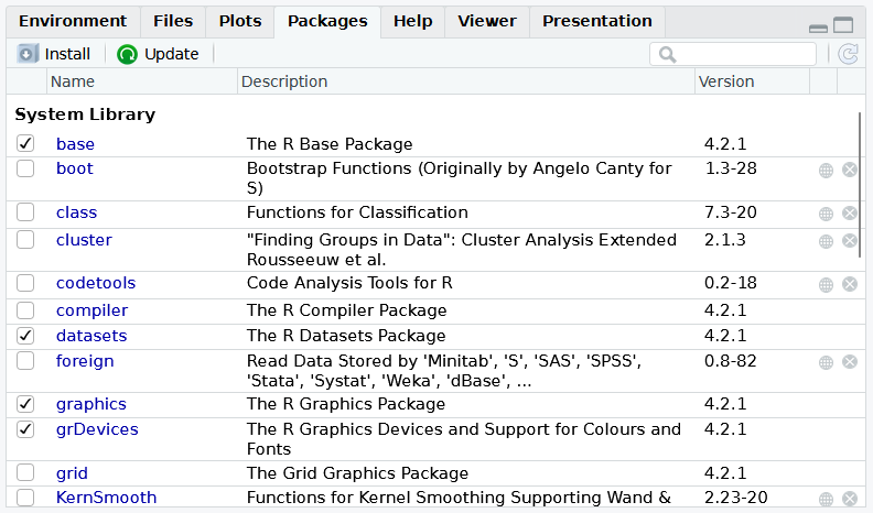
The packages which are currently loaded have a tick in the box next to them. A loaded package has its functions available to use without needing to specify the namespace.

For example if you try to use mutate() from the dplyr package without loading the library or using the namespace, you will receive an error.

mutate(df, new_col = 1:5)
#' Error in mutate(df, new_col = 1:5) : could not find function "mutate"

This can be fixed by using the namespace.

dplyr::mutate(df, new_col = 1:5)
#'   a b new_col
#' 1 a 1       1
#' 2 b 2       2
#' 3 c 3       3
#' 4 d 4       4
#' 5 e 5       5

Alternatively, loading the library means you no longer need to specify the namespace.

library(dplyr)
#' Attaching package: ‘dplyr’
#' 
#' The following objects are masked from ‘package:stats’:
#' 
#'     filter, lag
#' 
#' The following objects are masked from ‘package:base’:
#' 
#'     intersect, setdiff, setequal, union

mutate(df, new_col = 1:5)
#'   a b new_col
#' 1 a 1       1
#' 2 b 2       2
#' 3 c 3       3
#' 4 d 4       4
#' 5 e 5       5

You may have noticed the messages regards masked objects when loading dplyr. This happens because the base R packages contain functions with the same names as functions within the dplyr package.

filter() for example a function from the base library stats. When dplyr is loaded it masks the stats version, so a call to filter() actually uses dplyr::filter() as opposed to stats::filter(). To make matters worse, they do not do the same thing.

This can lead to errors and mistakes and the topic is rather contentious. I generally recommend using the namespace for all none base functions, but if you have loaded dplyr and call filter(), it is still going to use the dplyr version.

The only real solution is to be aware of this potential issue, particularly when moving between different projects.

A very useful shortcut in RStudio CTRL + SHIFT + F10, restarts R, removes all objects from the environment, and unloads all packages. When moving between projects this is a convenient way to ensure you are starting afresh.

Help

The Help tab allows us to browse package and function documentation within RStudio. It’s an incredibly useful feature, allowing you to access the documentation for any function by using the search bar in the top right of the tab, or programmatically by prepending ‘?’ to a function name.

> ?print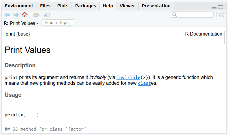

Environment

The Environment tab allows us to view all of the objects that exist in our global environment.

At this stage the differences are not important as they form part of a much broader topic, however, you can see that whilst both my_dbl and my_df are objects, their characteristics are very different, and it is those characteristics that determine how they are handled by functions and the ways in which we can manipulate them.

If two objects are created, user and df, they will appear in the environment tab.

user <- Sys.info()["user"]

df <- data.frame(a = letters[1:5], b = 1:5)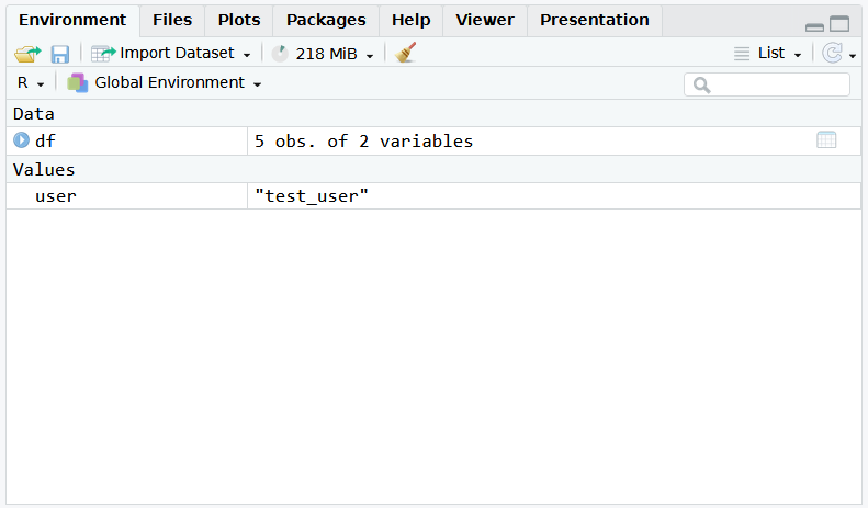

One of RStudios most useful features for data scientists and analysts working interactively is the ability to explore tabular data with the built in viewer.

The small icon that looks like a spreadsheet indicates that you can click on df in the environment pane to open the object in the viewer. The same can be achieved by running View(df).

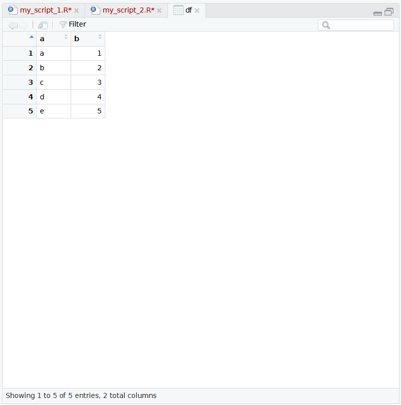
The viewer functionality is ideal for exploring data, checking results, and other interactions with tabular data. It can also be helpful for exploring the format of list objects, especially nested lists.

When working with larger datasets the viewers performance may become an issue. One solution to this is to use the head() function. head() returns the first parts of a vector, matrix, table, data frame, or function.

> View(head(df))

Objects in R

Everything that exists in R is an object. An object can have many characteristics recorded about it, and these characteristics control the way in which the object can be used and interacted with.

To further explore this concept lets look at an integer atomic vector and a data.frame, then use some functions to explore their characteristics.

my_dbl <- 1:10L

my_df <- data.frame(col_1 = 1:10)

# mode function
mode(my_dbl)
#' [1] "numeric"

mode(my_df)
#' [1] "list"

# typeof function
typeof(my_dbl)
#' [1] "integer"

typeof(my_df)
#' [1] "list"

# class function
class(my_dbl)
#' [1] "integer"

class(my_df)
#' [1] "data.frame"

# attributes function
attributes(my_dbl)
#' NULL

attributes(my_df)
#' $names
#' [1] "col_1"
#' 
#' $class
#' [1] "data.frame"
#' 
#' $row.names
#' [1]  1  2  3  4  5  6  7  8  9 10

Source

The Source pane provides RStudios text editing functionality. It is where you write, and edit code. It is also where the data viewer will open when using the View() function.

Running code

There are a few ways to run code written in the source pane.

CTRL + ENTER Runs the current line, or lines if the block of code spans more than just the single line. If you highlight a portion of code, it causes just the highlighted parts to run.

The Run button in the source pane tool bar functions in the same way as pressing CTRL + Enter.

It is possible to run entire scripts in this way by highlighting every line and clicking run, however, I would recommend using the keyboard shortcut CTRL + SHIFT + ENTER to run an entire script using source().

We can also run an entire script using the Source button.

RStudios documentation on the differences between Run and Source states;

The difference between running lines from a selection and invoking Source is that when running a selection all lines are inserted directly into the console whereas for Source the file is saved to a temporary location and then sourced into the console from there (thereby creating less clutter in the console).

Code executed with *Run*	Code executed with *Source*

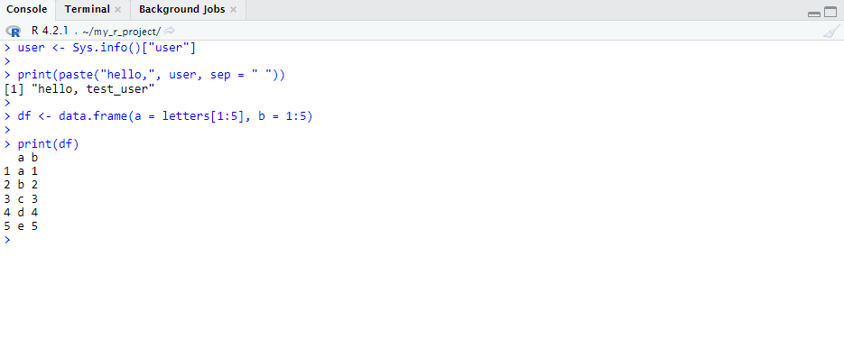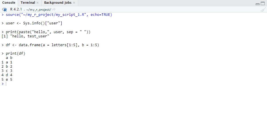Whilst there are some other subtle differences between running and sourcing code, it is sufficient in most cases to use whichever is easier for you.

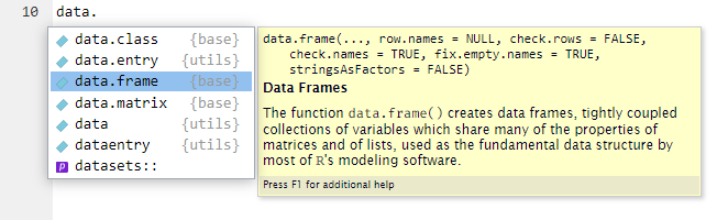
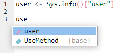
Code completion

RStudio provides support for code completion. For example, typing data. generates a context menu with some useful suggestions, and you can the arrow keys to navigate through them. If you find one that you wish to use, data.frame in this case, you press TAB to insert it and complete the code. This can be particularly useful if you partially remember a function name.

This also works for objects that have been created.

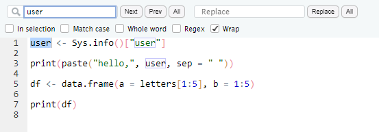
Find and replace

The small magnifying glass located on the source pane toolbar opens up the search and replace functionality. The keyboard shortcut CTRL + F can also be used.

Typing in the search box allows you to find all instances of a word throughout your script, and you can also replace occurrences of a word with an alternative. The functionality can be really useful, especially when working on large code bases.

Console

The Console pane allows commands to be written and executed immediately. It also shows the results of code that has been ran or sourced from the source pane.

If you want to check the current working directory for example, you could type getwd() in an open R script, run the line of code, check the output in the console, and finally delete the the getwd() function from the script. Alternatively, you can type getwd() into the console directly and hit Enter.

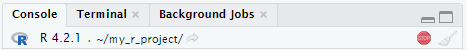
Whilst code is running, you will notice a red stop sign icon in the upper right of the console pane. This is a useful indicator that R is running code, and clicking it will attempt to interrupt the current process.

The small broom icon clears all text from the console.

The console also supports recalling previous commands using the arrow keys. Whilst using the console, tapping UP ARROW will retrieve the last command that was ran. You can browse through the available history using the arrow keys.

Terminal

The terminal pane allows access to the system shell, the underlying operating system. The functionality that this provides will largely depend on the OS you are running RStudio on top of, but common use cases include using Git for version control, and remote system management.

Plots

The Plots pane allows you to view plots you have created.

hist(rnorm(100))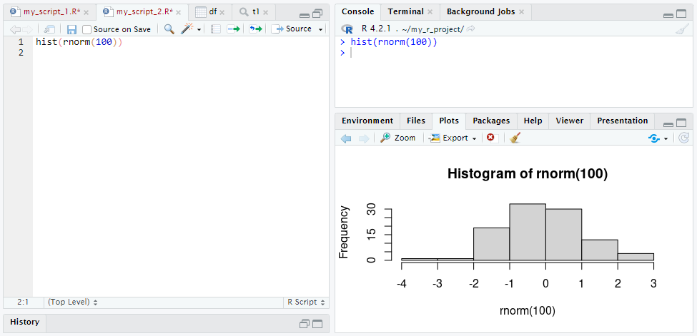

The Plots pane toolbar provides a few useful functions. The Zoom button opens the plot in a larger pop-out. The Export button provides options to export the plot as an image or pdf, and also allows you to copy the plot to the clipboard.

Next steps

RStudio is a powerful and popular IDE for use with R. It also supports python, making it a good choice as a development environment for data science.

Getting familiar with RStudio often allows users to perform work more efficiently through learning how to make use of the functionality that it provides. Playing around with the layout and appearance can also prove beneficial in creating an environment that is pleasant to work in.

PREVIOUSMaking R Scripts Executable on Linux

NEXTR Basics - Packages