Data frames are a fundamental part of R and the functionality they provide plays an integral role in many analysis and data science based workflows. Data frames are rectangular, 2 dimensional table structures, resembling rows and columns which makes them flexible and intuitive to work with.
Creating a data.frame
Many functions commonly used to read tabular data into R will by default return a data.frame. We can also use the ``data.frame() function to create a data.frame with any number of columns. Imagine that you have the names, ages, and postcodes of 5 people. A data.frame with 5 rows and 3 columns would be an ideal way to store this information.
data.frame(
  name = c("Alan", "Harry", "Frances", "Polly", "Walt"),
  age = c(48, 34, 78, 45, 21),
  postcode = c("ab123a", "cd123a", "ef123a", "gh123a", "ij123a")
)

#'      name  age postcode
#' 1    Alan   48   ab123a
#' 2   Harry   34   cd123a
#' 3 Frances   78   ef123a
#' 4   Polly   45   gh123a
#' 5    Walt   21   ij123a
The only constraint when creating a data.frame is that the columns must be of the same length, otherwise an error is returned.
data.frame(
    name = c("Alan", "Harry"),
    age = c(48, 34, 78, 45, 21),
    postcode = c("ab123a", "cd123a", "ef123a", "gh123a", "ij123a")
)

#' Error in data.frame(name = c("Alan", "Harry"), age = c(48, 34, 78, 45,  :
#'   arguments imply differing number of rows: 2, 5
Each column of a data.frame is actually a vector, so we can also construct a data.frame from vectors, as long as they are of equal length.
name_vector <- c("Alan", "Harry", "Frances", "Polly", "Walt")
age_vector <- c(48, 34, 78, 45, 21)
postcode_vector <- c("ab123a", "cd123a", "ef123a", "gh123a", "ij123a")

df <- `data.frame`(
  name = name_vector,
  age = age_vector,
  postcode = postcode_vector
)

print(df)
#'      name  age postcode
#' 1    Alan   48   ab123a
#' 2   Harry   34   cd123a
#' 3 Frances   78   ef123a
#' 4   Polly   45   gh123a
#' 5    Walt   21   ij123a
data.frame columns
As data.frame columns are vectors we can access them and use them inside functions that accept vectors. There are a few different ways to access a data.frame column, but the 3 most common are;
- Using the
$operator. - Using the index.
- Using the column name.
# using $
df$age
#' [1] 48 34 78 45 21

# using the index
df[2]
#'   age
#' 1  48
#' 2  34
#' 3  78
#' 4  45
#' 5  21

# using the column name
df["age"]
#'   age
#' 1  48
#' 2  34
#' 3  78
#' 4  45
#' 5  21
You will notice that options 2 & 3 returned the column in a different format. Using $ stripped the column of it’s data.frame attributes, whereas the other methods retained them. You can check this by using typeof() and attributes() on df$age and df["age"].
typeof(df$age)
#' [1] "double"

typeof(df["age"])
#' [1] "list"

attributes(df$age)
#' NULL

attributes(df["age"])
#' $names
#' [1] "age"
#'
#' $row.names
#' [1] 1 2 3 4 5
#'
#' $class
#' [1] "data.frame"
The output of typeof(df["age"]) may have surprised you slightly. Beneath the surface, data.frame’s are actually list objects with each column forming an element of the list.
For now, we will focus on using the $ operator to access columns. The other options can be useful at times, though as a general rule try to avoid option 2 (df[2]). Specifying column names explicitly makes your code simpler to comprehend,improves reproducibility, and helps to reduce errors if your data changes.
Accessing a column allows us to use it as we would any other vector. We can get the sum and mean of the age column with the appropriate functions.
sum(df$age)
#' [1] 226

mean(df$age)
#' [1] 45.2
We can also subset a column accessed with the $ operator using the index system.
# get the 1st element of df$age
df$age[1]

#' [1] 48

# get the 1st 3 elements of df$age
df$age[1:3]

#' [1] 48 34 78

# get the last 3 elements of df$age programmatically
len <- length(df$age)

df$age[(len-2):len]

#' [1] 78 45 21
data.frame subsets
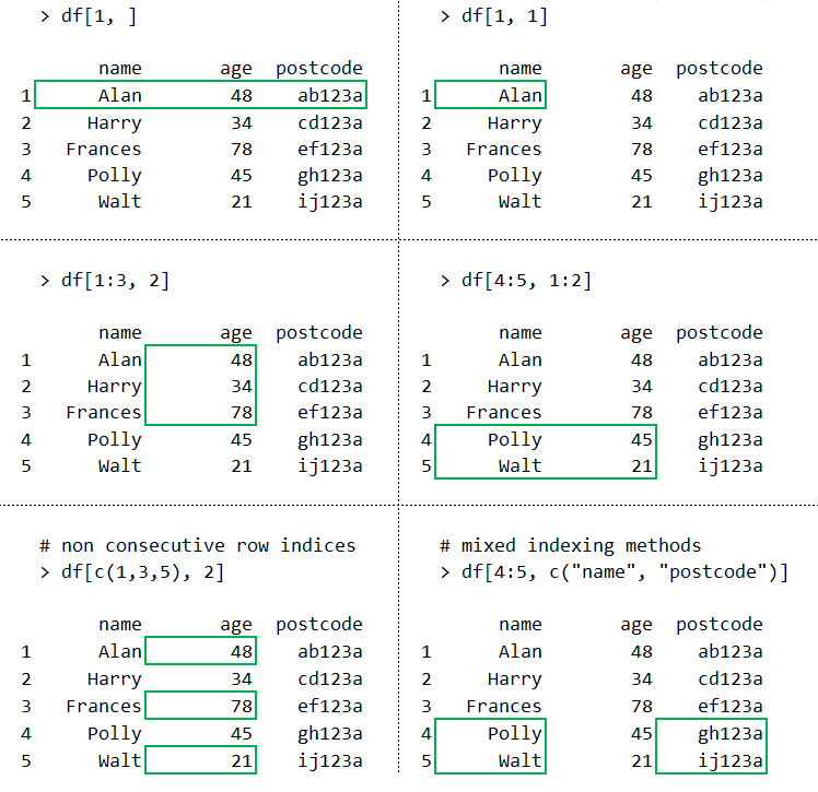
We can also create subsets of data.frame’s using indices. With data.frame’s, two indices are provided, the first for the rows and the second for the columns. Blank indices are also acceptable, as long as they are separated with ,.
Each individual element in a data.frame has 2 indices.
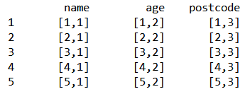
The below examples show how the index system can be used to access various elements in our data.frame.
Functions for data.frame’s
When working with vectors we can check their length using the length() function. Given that all columns of a data.frame are vectors of equal length we could use length() on any column, however, it is more convenient to use the nrow() function to identify the number of rows.
nrow(df)

#' [1] 5
Some other useful functions for interacting with data.frame’s include ncol(), used to get the number of columns, and names(), which provides the names of the data.frame’s columns.
ncol(df)

#' [1] 3

names(df)

#' [1] "name"     "age"
#' [3] "postcode"
The names() function can also be used to change the names of columns.
names(df) <- c("first_name", "cur_age", "pcode")

#'   first_name cur_age  pcode
#' 1       Alan      48 ab123a
#' 2      Harry      34 cd123a
#' 3    Frances      78 ef123a
#' 4      Polly      45 gh123a
#' 5       Walt      21 ij123a
Next steps
data.frame’s are one of the most useful data structures in R and the fact that this functionality is built into the language is one of the reasons that R is an excellent choice for statistics, analysis, and data science.
To put some of the key points above into practice, try the following tasks.
Try creating a data.frame named “my_df” with 3 columns named “col_a”, “col_b”, and “col_c”.
“col_a” should contain the first 10 letters of the alphabet as individual elements.
“col_b” should contain the numbers 1 to 10.
“col_c” should contain the numbers 11 to 20, but in reverse.
Your resulting data.frame should look like this;
print(my_df)
#'    col_a col_b col_c
#' 1      a     1    20
#' 2      b     2    19
#' 3      c     3    18
#' 4      d     4    17
#' 5      e     5    16
#' 6      f     6    15
#' 7      g     7    14
#' 8      h     8    13
#' 9      i     9    12
#' 10 j 10 11-
What is the product of the sum of col_b and col_c?
-
What is the sum of all values in col_b and col_c?
-
What is the sum of all values in col_b and col_c, but considering only the first 5 rows of my_df?
Answers
1. 85252. 210
3. 105