In Data Frames Part 1 we looked at creating data.frame objects, accessing their columns, and creating subsets of them using their row and column indices. We also looked at some useful functions for interacting with data.frame objects’s, including ncol(), nrow(), and names().
In the 2nd part we explore these key data structures in more detail.
Working with data frames
mtcars is one of a variety of data sets that are included with R and are typically used in tutorials. We can view the first few rows of mtcars to get a feel for the data set using the head() function.
head(mtcars)
#'                    mpg cyl disp  hp drat    wt  qsec vs am gear carb
#' Mazda RX4         21.0   6  160 110 3.90 2.620 16.46  0  1    4    4
#' Mazda RX4 Wag     21.0   6  160 110 3.90 2.875 17.02  0  1    4    4
#' Datsun 710        22.8   4  108  93 3.85 2.320 18.61  1  1    4    1
#' Hornet 4 Drive    21.4   6  258 110 3.08 3.215 19.44  1  0    3    1
#' Hornet Sportabout 18.7   8  360 175 3.15 3.440 17.02  0  0    3    2
#' Valiant           18.1   6  225 105 2.76 3.460 20.22  1  0    3    1
The tail() function can also be used to inspect an object and works similarly to head(), returning the last rows of a data.frame. head() and tail() can also be used on individual columns, or in fact any vector, to return the first (or last) few elements.
head(mtcars$mpg)
#` [1] 21.0 21.0 22.8 21.4 18.7 18.1
You may have noticed that mtcars doesn’t actually have a column containing the car names, rather they are stored as row names. We can check and confirm this using the row.names() function.
row.names(mtcars)
#' [1] "Mazda RX4"           "Mazda RX4 Wag"
#' [3] "Datsun 710"          "Hornet 4 Drive"
#' [5] "Hornet Sportabout"   "Valiant"
#' ...
Subset rows based on criteria
We know that we can access a data.frame’s elements using the indices of the rows and columns that we want to include. You can revisit Data Frames Part 1 for a refresher.
The position of the row and column indices along with the , are perhaps the most important considerations at this stage, and are the most likely to cause confusion.
It is important to take extra care with the syntax initially, but as you gain experience from putting the theory into practice you will find that it quickly becomes more intuitive, for example, knowing that if we don’t include the comma and only pass one index (i.e. df[1]), R will assume that we want a column.
As you become more confident with manipulating data.frame objects in this way you can start to advance towards more powerful applications to create specific subsets of data.frame’s.
Subset rows using a numeric vector
Lets say that we want to extract all of the rows from mtcars for cars with over 200 horsepower.
To achieve our goal we could look at mtcars and write down the row numbers where the value in the hp column is greater than 200, which would be rows 7, 15, 16, 17, 24, 29, and 31.
Using the index system we are able to create a subset of mtcars containing those rows.
mtcars[c(7, 15, 16, 17, 24, 29, 31), ]
#'                      mpg cyl disp  hp drat    wt  qsec vs am gear carb
#' Duster 360          14.3   8  360 245 3.21 3.570 15.84  0  0    3    4
#' Cadillac Fleetwood  10.4   8  472 205 2.93 5.250 17.98  0  0    3    4
#' Lincoln Continental 10.4   8  460 215 3.00 5.424 17.82  0  0    3    4
#' Chrysler Imperial   14.7   8  440 230 3.23 5.345 17.42  0  0    3    4
#' Camaro Z28          13.3   8  350 245 3.73 3.840 15.41  0  0    3    4
#' ...
Note that we have used the c() function to create a vector containing the row numbers, and we have included the , even though we aren’t specifying any columns. If we try to select the rows without including the ,, R will assume we want columns, and since we only have 11 columns will return an error.
mtcars[c(7, 15, 16, 17, 24, 29, 31)]
#' Error in `[.data.frame`(mtcars, c(7, 15, 16, 17, 24, 29, 31)) :
#' undefined columns selected
Whilst this approach works, its clearly not very scalable. It requires manually counting the rows we want and would be impractical with larger or more complex data sets.
One way to approach the problem in a programmatic way is to use the which() function.
hp_200 <- which(mtcars$hp > 200)

print(hp_200)
#' [1]  7 15 16 17 24 29 31
which(mtcars$hp > 200) has returned the indices of elements with values greater than 200 in the mtcars hp column. We have assigned the output of which() to hp_200, so we can now reuse those values elsewhere, in this case to subset our data.frame.
mtcars[hp_200, ]
#'                      mpg cyl disp  hp drat    wt  qsec vs am gear carb
#' Duster 360          14.3   8  360 245 3.21 3.570 15.84  0  0    3    4
#' Cadillac Fleetwood  10.4   8  472 205 2.93 5.250 17.98  0  0    3    4
#' Lincoln Continental 10.4   8  460 215 3.00 5.424 17.82  0  0    3    4
#' Chrysler Imperial   14.7   8  440 230 3.23 5.345 17.42  0  0    3    4
#' Camaro Z28          13.3   8  350 245 3.73 3.840 15.41  0  0    3    4
#' ...
It is possible to skip the step of assigning the output from which() altogether by using the function within [ ] directly.
mtcars[which(mtcars$hp > 200),]
#'                      mpg cyl disp  hp drat    wt  qsec vs am gear carb
#' Duster 360          14.3   8  360 245 3.21 3.570 15.84  0  0    3    4
#' Cadillac Fleetwood  10.4   8  472 205 2.93 5.250 17.98  0  0    3    4
#' Lincoln Continental 10.4   8  460 215 3.00 5.424 17.82  0  0    3    4
#' Chrysler Imperial   14.7   8  440 230 3.23 5.345 17.42  0  0    3    4
#' Camaro Z28          13.3   8  350 245 3.73 3.840 15.41  0  0    3    4
#' ...
Subset rows using a logical vector
We can also subset mtcars using a logical (TRUE or FALSE) vector. If we run mtcars$hp > 200 we get a logical vector in return, where TRUE indicates that the vector element was greater than 200.
mtcars$hp > 200

#'  [1] FALSE FALSE FALSE FALSE FALSE FALSE  TRUE FALSE FALSE FALSE FALSE
#' [12] FALSE FALSE FALSE  TRUE  TRUE  TRUE FALSE FALSE FALSE FALSE FALSE
#' [23] FALSE  TRUE FALSE FALSE FALSE FALSE  TRUE FALSE  TRUE FALSE
Logical vectors can be used to subset other vectors and data.frame’s. We can explore this in action with a simple example.
my_vector <- c("Alan", "Harry", "Frances", "Polly", "Walt")

logical_vector <- c(TRUE, FALSE, TRUE, FALSE, TRUE)

my_vector[logical_vector]

#' [1] "Alan" "Frances" "Walt"
The 1st, 2nd, and 3rd elements of logical_vector are TRUE, so the subset operation keeps the 1st, 2nd, and 3rd elements of my_vector. We can use this approach with mtcars to create the subset data.frame of cars with over 200 hp.
mtcars[mtcars$hp > 200, ]
#'                      mpg cyl disp  hp drat    wt  qsec vs am gear carb
#' Duster 360          14.3   8  360 245 3.21 3.570 15.84  0  0    3    4
#' Cadillac Fleetwood  10.4   8  472 205 2.93 5.250 17.98  0  0    3    4
#' Lincoln Continental 10.4   8  460 215 3.00 5.424 17.82  0  0    3    4
#' Chrysler Imperial   14.7   8  440 230 3.23 5.345 17.42  0  0    3    4
#' Camaro Z28          13.3   8  350 245 3.73 3.840 15.41  0  0    3    4
#' ...
R often provides us with lots of ways to do the same thing. Which approach you use will often come down to how the wider project is structured and choosing an approach is something that becomes more intuitive with experience. Considerations such as readability and how obvious the functionality of a piece of code is to a third party, or indeed yourself upon returning to it, are important.
For newcomers it is often best to work with the option you find most intuitive, but in essence all of these approaches give you the same output.
method_a <- mtcars[c(7, 15, 16, 17, 24, 29, 31), ]

method_b <- mtcars[which(mtcars$hp > 200), ]

method_c <- mtcars[mtcars$hp > 200, ]

identical(method_a, method_b)
#' [1] TRUE

identical(method_b, method_c)
#' [1] TRUE
A tidy approach
Use of the tidyverse is somewhat ubiquitous in R and the tidy style is now often taught before base R. You will notice that so far we haven’t looked at any tidy functions. Whilst the tidyverse posits itself as being simpler to learn, this isn’t necessarily true. Building a strong understanding of base R will afford you greater flexibility and comprehension of the language when progressing to more advanced usage.
With that in mind, it can be useful to see how the examples we have looked at so far might translate into the tidyverse. The example below demonstrates how we could produce a subset data.frame of cars with over 200 hp from mtcars in a tidy fashion.
library(dplyr)
mtcars %>%
dplyr::filter(hp > 200)
#' mpg cyl disp hp drat wt qsec vs am gear carb
#' Duster 360 14.3 8 360 245 3.21 3.570 15.84 0 0 3 4
#' Cadillac Fleetwood 10.4 8 472 205 2.93 5.250 17.98 0 0 3 4
#' Lincoln Continental 10.4 8 460 215 3.00 5.424 17.82 0 0 3 4
#' Chrysler Imperial 14.7 8 440 230 3.23 5.345 17.42 0 0 3 4
#' Camaro Z28 13.3 8 350 245 3.73 3.840 15.41 0 0 3 4
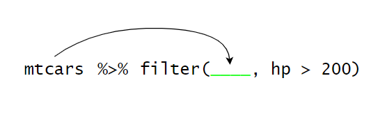
#' ...You will notice the use of the pipe operator %>% and that the hp column is referred to simply as hp rather than mtcars$hp. The dplyr functions try to be more intuitive by assuming hp in this instance will be a column in mtcars.
A (very) brief note about pipes: Pipes are commonly used in R to chain together multiple functions. There is also a native pipe operator in R |> (available in versions 4.1.0 and above). In its simplest usage the pipe operator takes the object to its left and passes it to its right as the first argument.
In the example above, the pipe operator takes mtcars and passes it to the first argument of dplyr::filter().
We can write the snippet without pipes, whilst still using dplyr::filter().
mtcars %>% dplyr::filter(hp > 200)

# is equivalent to

dplyr::filter(mtcars, hp > 200)
Base or tidy? A natural question to arise whilst learning R is whether to prefer base R or tidy R. As you become comfortable with the language you will likely develop a preference for approaching problems in a certain way and may find that you prefer one framework over another.
However, an either or approach is only likely to lead to problems down the line. Whilst learning the language it is preferable to be exposed to multiple approaches in order that you can understand code written by others and be aware of alternatives if you encounter a challenging problem.
Subset columns based on criteria
We can select a subset of columns from mtcars in a few different ways.
Subset columns using a numeric vector
We can select columns using their indices. We don’t need to include , within [ ] if we only want columns. However, it doesn’t cause any issues if we do include ,, but it must come before the column indices. If we want to select the first 3 columns of mtcars we can use a numeric vector.
mtcars[1:3]
#'                      mpg cyl  disp
#' Mazda RX4           21.0   6 160.0
#' Mazda RX4 Wag       21.0   6 160.0
#' Datsun 710          22.8   4 108.0
#' Hornet 4 Drive      21.4   6 258.0
#' Hornet Sportabout   18.7   8 360.0

identical(mtcars[, 1:3], mtcars[1:3])
#' [1] TRUE

identical(mtcars[1:3, ], mtcars[1:3])
#' [1] FALSE
You will have noticed in the example above that mtcars[, 1:3] and mtcars[1:3] return the same object, but mtcars[1:3, ] doesn’t. The position of the , in mtcars[1:3, ] causes R to extract the first 3 rows, rather than columns.
Subset columns using a character vector
We can use the column names to access specific columns of mtcars. The names() function can be really helpful here and allows us to check the name values that are available.
names(mtcars)
#'  [1] "mpg"  "cyl"  "disp" "hp"   "drat" "wt"   "qsec" "vs"   "am"   "gear" "carb"
Lets use the column names to extract the mpg, cyl, and hp columns from mtcars.
mtcars[c("mpg", "cyl", "hp")]
#'                      mpg cyl  hp
#' Mazda RX4           21.0   6 110
#' Mazda RX4 Wag       21.0   6 110
#' Datsun 710          22.8   4  93
#' Hornet 4 Drive      21.4   6 110
#' Hornet Sportabout   18.7   8 175
#' ...
This approach is effective and straight forward to use, making it an ideal approach for creating subsets of specific columns.
Subset columns using a logical vector
Sometimes you may want to select columns in a more dynamic way. Lets say we want a data.frame consisting of any column from mtcars with a name that is 2 characters long.
We can first get the number of characters in each of the column names and store the vector as name_len.
name_len <- nchar(names(mtcars))

print(name_len)
#' [1] 3 3 4 2 4 2 4 2 2 4 4
We then convert the name_len numeric vector to logical one.
name_len <- name_len == 2

print(name_len)
 [1] FALSE FALSE FALSE  TRUE FALSE TRUE FALSE  TRUE  TRUE FALSE FALSE
Finally, we can use name_len to select all of the columns from mtcars with names 2 characters long.
mtcars[name_len]
#'                      hp    wt vs am
#' Mazda RX4           110 2.620  0  1
#' Mazda RX4 Wag       110 2.875  0  1
#' Datsun 710           93 2.320  1  1
#' Hornet 4 Drive      110 3.215  1  0
#' Hornet Sportabout   175 3.440  0  0
#' ...
As with our examples above, we can also avoid the intermediate steps by refactoring our code into a concise one-liner.
mtcars[nchar(names(mtcars)) == 2]

#'                      hp    wt vs am
#' Mazda RX4           110 2.620  0  1
#' Mazda RX4 Wag       110 2.875  0  1
#' Datsun 710           93 2.320  1  1
#' Hornet 4 Drive      110 3.215  1  0
#' Hornet Sportabout   175 3.440  0  0
#' ...
Subset rows and columns simultaneously based on criteria
We can combine what we have looked at so far to create a subset of both columns and rows from mtcars. To extract the mpg, cyl, and hp columns from mtcars, but only keeping rows where hp is greater than 200, we can combine the mtcars[mtcars$hp > 200,] and mtcars[c("mpg", "cyl", "hp")] code snippets we used earlier.
At this point we also need to remember the order in which we specify rows and columns inside [ ].
Lets give it a try, providing our row subset criteria followed by our column subset criteria.
mtcars[mtcars$hp > 200, c("mpg", "cyl", "hp")]
#'                      mpg cyl  hp
#' Duster 360          14.3   8 245
#' Cadillac Fleetwood  10.4   8 205
#' Lincoln Continental 10.4   8 215
#' Chrysler Imperial   14.7   8 230
#' Camaro Z28          13.3   8 245
#' ...
We can also select rows based on the values in a column that we don’t want to actually include in our output. For example, if we want the mpg, cyl, and hp columns from mtcars, where carb is greater than 4, we don’t actually need to include carb in our new data.frame.
mtcars[mtcars$carb > 4, c("mpg", "cyl", "hp")]
#'                mpg cyl  hp
#' Ferrari Dino  19.7   6 175
#' Maserati Bora 15.0   8 335
A tidy approach
Examples of a tidyverse approach to creating a subset of rows and columns simultaneously.
library(dplyr)

mtcars %>%
  dplyr::filter(hp > 200) %>%
  dplyr::select(mpg, cyl, hp)
#'                      mpg cyl  hp
#' Duster 360          14.3   8 245
#' Cadillac Fleetwood  10.4   8 205
#' Lincoln Continental 10.4   8 215
#' Chrysler Imperial   14.7   8 230
#' Camaro Z28          13.3   8 245
#' ...

mtcars %>%
  dplyr::filter(carb > 4) %>%
  dplyr::select(mpg, cyl, hp)
#'                mpg cyl  hp
#' Ferrari Dino  19.7   6 175
#' Maserati Bora 15.0   8 335
& AND | OR
The logical & (AND) and | (OR) operators are very important in any programming language, allowing us to build logic based on multiple conditions. The following examples demonstrate the returns generated by using the logical operators in different situations.
TRUE & TRUE
#' [1] TRUE

TRUE & FALSE
#' [1] FALSE

FALSE & FALSE
#' [1] FALSE

TRUE & TRUE & TRUE
#' [1] TRUE

TRUE & TRUE & FALSE
#' [1] FALSE

TRUE | FALSE
#' [1] TRUE

TRUE | TRUE
#' [1] TRUE

FALSE | FALSE
#' [1] FALSE

TRUE | FALSE | FALSE
#' [1] TRUE
In one of the examples above we returned rows from mtcars where the hp value was greater than 200 and the carb value was greater than 4. We can combine the separate criteria to return rows where both conditions are TRUE using the & operator.
mtcars[mtcars$carb > 4 & mtcars$hp > 200, ]
#'               mpg cyl disp  hp drat   wt qsec vs am gear carb
#' Maserati Bora  15   8  301 335 3.54 3.57 14.6  0  1    5    8
We can also return the rows of mtcars where either of the conditions are TRUE.
mtcars[mtcars$carb > 4 | mtcars$hp > 200, ]
#'                      mpg cyl disp  hp drat    wt  qsec vs am gear carb
#' Duster 360          14.3   8  360 245 3.21 3.570 15.84  0  0    3    4
#' Cadillac Fleetwood  10.4   8  472 205 2.93 5.250 17.98  0  0    3    4
#' Lincoln Continental 10.4   8  460 215 3.00 5.424 17.82  0  0    3    4
#' Chrysler Imperial   14.7   8  440 230 3.23 5.345 17.42  0  0    3    4
#' Maserati Bora       15.0   8  301 335 3.54 3.570 14.60  0  1    5    8
#' ...
Using a single column from a data.frame subset
We might not always want to create a new data.frame, perhaps we simply want to know how many rows fulfil a certain criteria. We can use the nrow() function for this.
nrow(mtcars[mtcars$carb > 4,])
#' [1] 2

nrow(mtcars[mtcars$carb > 4 & mtcars$hp > 200, ])
#' [1] 1

nrow(mtcars[mtcars$carb > 4 | mtcars$hp > 200, ])
#' [1] 8
We can also apply this approach to more complex problems. If we want to know the mean value of disp where the value of carb is greater than 2 and hp is greater than 200, we could subset mtcars and then use mean() on the disp column.
new_mtcars <- mtcars[mtcars$carb > 2 & mtcars$hp > 200, ]

mean(new_mtcars$disp)
[1] 390.5714
However, we don’t actually need to go through the assignment step, rather we can access the column directly by placing the $ operator at the end of our subset syntax.
# to return the column as a vector
mtcars[mtcars$carb > 2 & mtcars$hp > 200, ]$disp
[1] 360 472 460 440 350 351 301
# to calculate the mean of the column
mean(mtcars[mtcars$carb > 2 & mtcars$hp > 200, ]$disp)
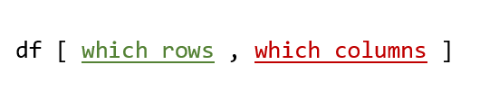
[1] 390.5714Missing commas: There are a few common ‘gotchas’ that tend to come up in this topic area. When using [ ] with data.frame objects the most common cause of errors is a misplaced or missing ,.
// specifying rows and columns requires a comma; rows then comma then columns
df [ which rows , which columns ]

// specifying columns only; no comma required OR comma then columns
df [ which columns ]   OR    df [ , which columns ]

// specifying rows only requires a comma; rows then comma
df [ which rows , ]
NA values: When using functions like sum() and mean() you may encounter situations where you have missing values within the vector you are applying the function to, which results in an output of NA.
sum(c(1,2,3,NA,5))
[1] NA
Many functions, including sum() and mean(), have an argument to allow missing values to be removed from consideration.
sum(c(1,2,3,NA,5), na.rm = TRUE)
[1] 11
To check the arguments available for a function you can use ? to access the functions documentation, for example ?sum.
There are a few ways to check for missing values in a vector, but a simple one is to use any() with is.na().
any(is.na(c(1,2,3,NA,5)))
[1] TRUE
A tidy approach
Example of a tidyverse approach to using a single column from a data.frame subset.
mtcars %>%
  dplyr::filter(carb > 2 & hp > 200) %>%
  dplyr::pull(disp) %>%
  mean
#' [1] 390.5714
Next steps
Manipulating data.frame objects is typically a fundamental part of any analytical or statistical workflow using R. The techniques described above are highly flexible and can be easily adapted to form part of a solution to many problems you might encounter.
You will also be starting to see how we can build more complex code from simpler component parts, such as placing code to produce a subset of a data.frame inside a function, for example sum(df[df$col_a == "x",]$col_b).
Practice and experimentation is key in regards to this topic and it is highly recommended that you play around with some data to fully explore it. You can also try some of the tasks below.
airquality is a dataset that comes with R, and is available by default.
-
airqualitycontains aMonthandDaycolumn, both of which are numeric (hint January = 1, February = 2, etc). What was the average temperature (Temp) during the month of July? -
What was the average wind speed (
Wind) during the first 10 days of the month of June? -
Calculate the sum of Ozone values from days where the Wind was greater then 10 OR the Temp was greater than 90 (hint
Ozonecontains some missing values).
Answers
1. 83.903232. 10.84
3. 2273